2 Step by Step: Demand Functions, Substitution Effect and Income Effect
2.1 Setup
A consumer chooses a bundle \((x, y)\) of two goods. Prices are \(p_x\) and \(p_y\) and income is \(I\). The budget constraint is:
\[p_x\,x + p_y\,y = I\]
The demand function for each good is the optimal quantity of that good as a function of prices and income:
\[x(p_x, p_y, I) \qquad\qquad y(p_x, p_y, I)\]
Three preferences:
\[u = x^{1/3}y^{2/3} \qquad\quad u = \tfrac13 x + \tfrac23 y \qquad\quad u = \min\left\{\tfrac13 x,\ \tfrac23 y\right\}\]
2.2 Demand functions. Cobb-Douglas: \(u = x^{1/3}y^{2/3}\)
2.2.1 Tangency condition
Marginal utilities:
\[MU_x = \tfrac13 x^{-2/3}y^{2/3} \qquad\qquad MU_y = \tfrac23 x^{1/3}y^{-1/3}\]
Dividing:
\[MRS = \frac{MU_x}{MU_y} = \frac{y}{2x}\]
Setting equal to \(p_x/p_y\):
\[\frac{y}{2x} = \frac{p_x}{p_y} \;\;\Longrightarrow\;\; p_y\,y = 2\,p_x\,x\]
2.2.2 Demand functions
Substituting \(p_y\,y = 2\,p_x\,x\) into the budget constraint:
\[p_x\,x + 2\,p_x\,x = I\]
Solving:
\[x(p_x, p_y, I) = \frac{I}{3\,p_x} \qquad\qquad y(p_x, p_y, I) = \frac{2I}{3\,p_y}\]
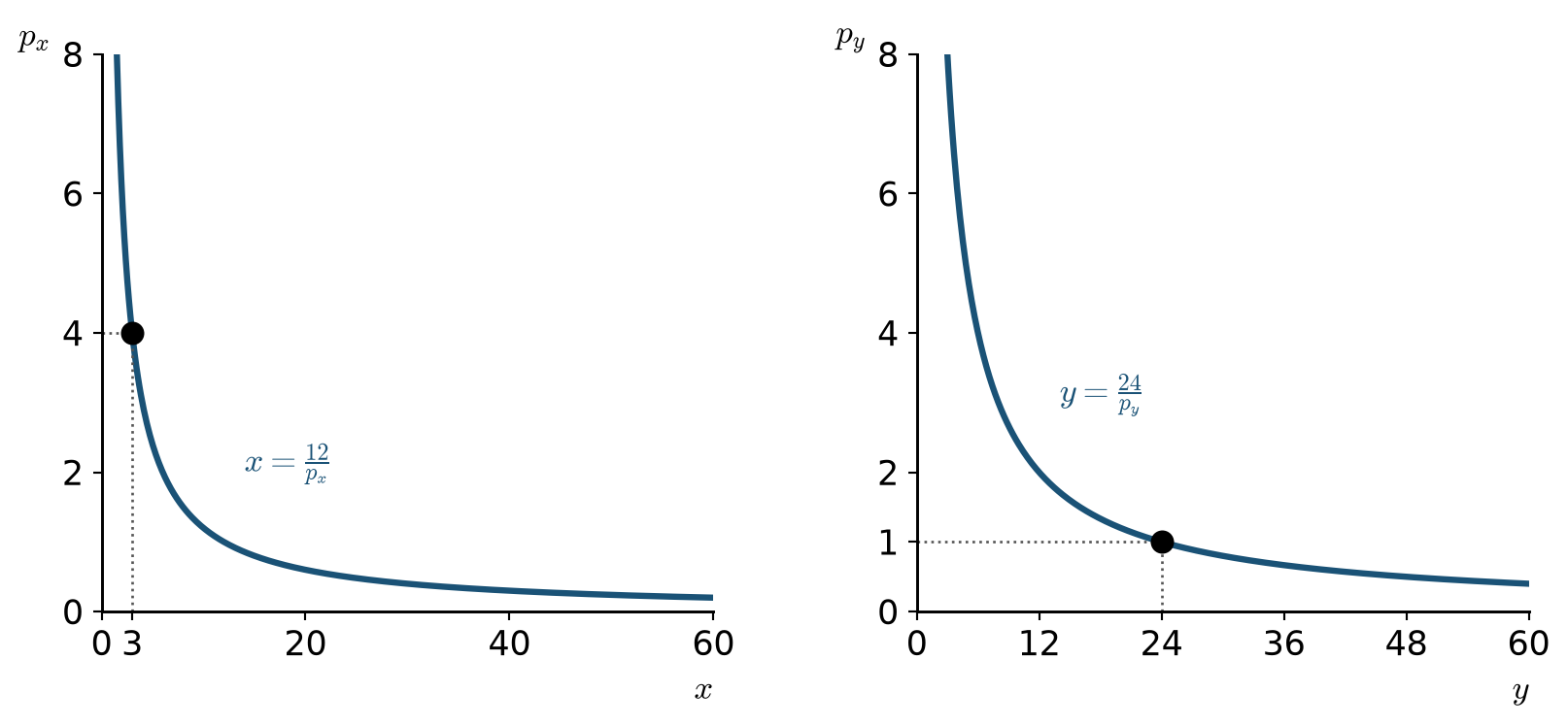
2.2.3 Demand curves
With \(I = 36\):
\[x = \frac{36}{3\,p_x} = \frac{12}{p_x} \qquad\qquad y = \frac{2\cdot 36}{3\,p_y} = \frac{24}{p_y}\]
2.3 Demand functions. Perfect substitutes: \(u = \tfrac13 x + \tfrac23 y\)
2.3.1 Comparing \(MRS\) and \(p_x/p_y\)
Marginal utilities:
\[MU_x = \tfrac13 \qquad\qquad MU_y = \tfrac23\]
Dividing:
\[MRS = \frac{1/3}{2/3} = \frac12\]
Comparing with \(p_x/p_y\):
\[\frac{p_x}{p_y} > \frac12 \;\;\Longrightarrow\;\; x = 0 \qquad\qquad \frac{p_x}{p_y} < \frac12 \;\;\Longrightarrow\;\; y = 0\]
2.3.2 Demand functions
Substituting into the budget constraint:
\[x(p_x, p_y, I) = \begin{cases} 0 & \tfrac{p_x}{p_y} > \tfrac12 \\[6pt] \dfrac{I}{p_x} & \tfrac{p_x}{p_y} < \tfrac12 \end{cases} \qquad\qquad y(p_x, p_y, I) = \begin{cases} \dfrac{I}{p_y} & \tfrac{p_x}{p_y} > \tfrac12 \\[6pt] 0 & \tfrac{p_x}{p_y} < \tfrac12 \end{cases}\]
If \(\tfrac{p_x}{p_y} = \tfrac12\), any bundle on the budget constraint is optimal.
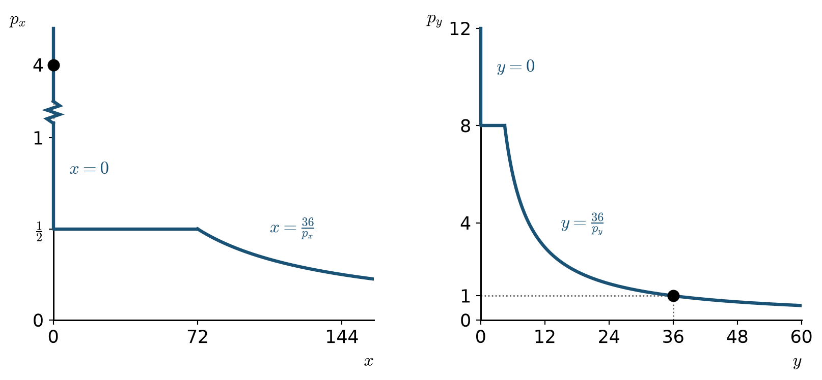
2.3.3 Demand curves
With \(I = 36\) and \(p_y = 1\):
\[x = \begin{cases} 0 & p_x > \tfrac12 \\[6pt] \dfrac{36}{p_x} & p_x < \tfrac12 \end{cases}\]
With \(I = 36\) and \(p_x = 4\):
\[y = \begin{cases} \dfrac{36}{p_y} & p_y < 8 \\[6pt] 0 & p_y > 8 \end{cases}\]
2.4 Demand functions. Perfect complements: \(u = \min\left\{\tfrac13 x,\ \tfrac23 y\right\}\)
2.4.1 Fixed-proportions condition
Without wasting either good:
\[\tfrac13 x = \tfrac23 y \;\;\Longrightarrow\;\; x = 2y\]
2.4.2 Demand functions
Substituting \(x = 2y\) into the budget constraint:
\[p_x\cdot 2y + p_y\,y = I\]
Solving:
\[y(p_x, p_y, I) = \frac{I}{2\,p_x + p_y} \qquad\qquad x(p_x, p_y, I) = \frac{2I}{2\,p_x + p_y}\]
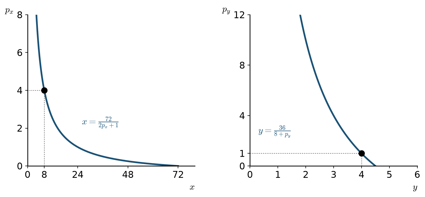
2.4.3 Demand curves
With \(I = 36\) and \(p_y = 1\):
\[x = \frac{72}{2\,p_x + 1}\]
With \(I = 36\) and \(p_x = 4\):
\[y = \frac{36}{8 + p_y}\]
2.5 Change in the price of \(x\)
The price of \(x\) falls. Income and the price of \(y\) do not change:
\[p_x = 4 \;\longrightarrow\; p_x' = \tfrac14 \qquad\qquad p_y = 1 \qquad\qquad I = 36\]
Three bundles:
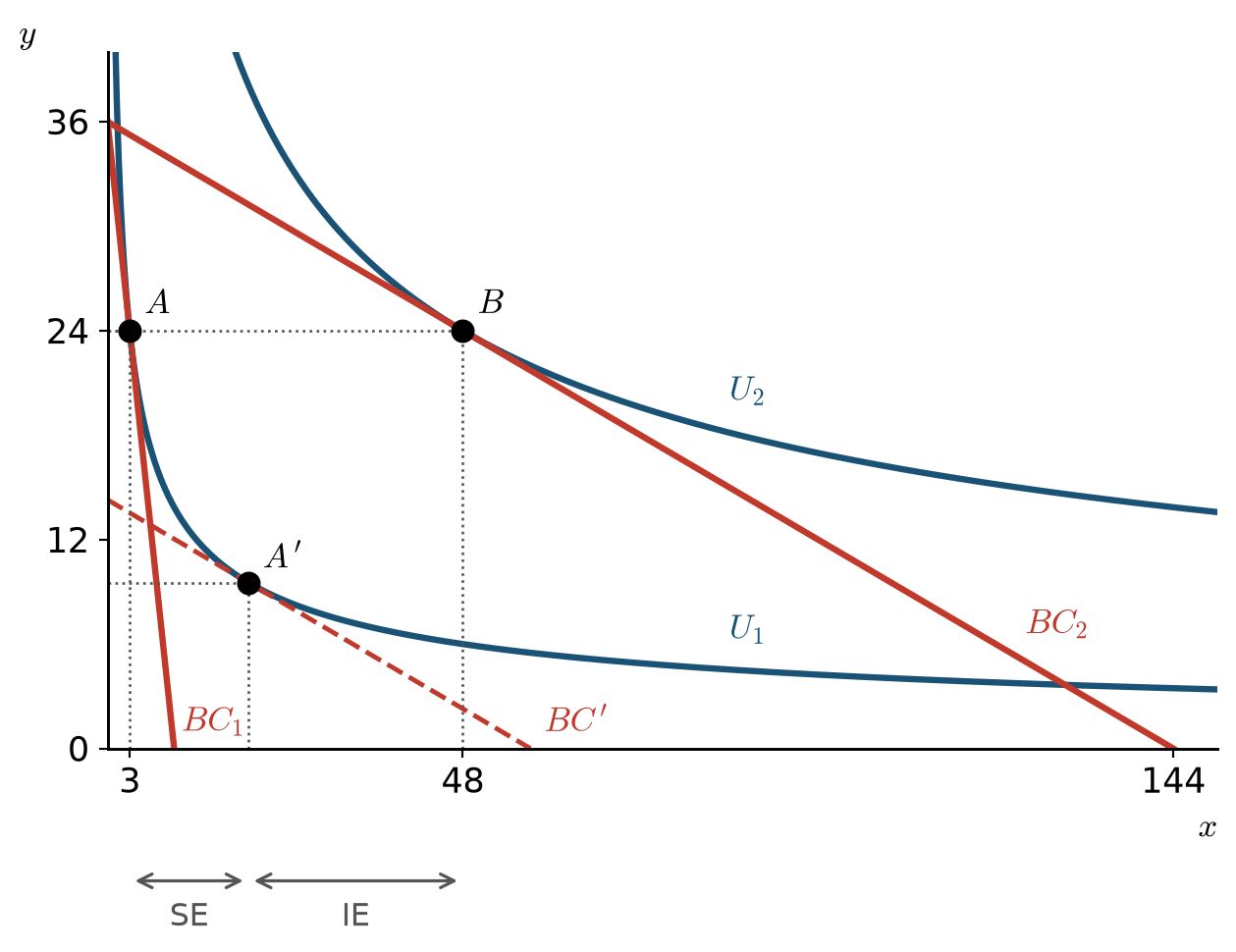
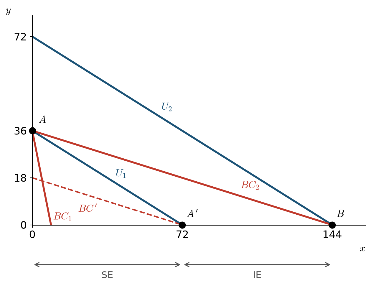
- \(A\): optimal bundle at the initial price, with utility \(U_1\).
- \(B\): optimal bundle at the final price, with utility \(U_2\).
- \(A'\): optimal bundle at the final price that keeps the initial utility \(U_1\).
Three budget constraints: \(BC_1\) (initial price), \(BC_2\) (final price) and \(BC'\) (parallel to \(BC_2\), through \(A'\)).
Effects on the quantity of \(x\):
\[SE = x_{A'} - x_A\]
\[IE = x_B - x_{A'}\]
\[TE = x_B - x_A = SE + IE\]
2.6 Substitution and income effects. Cobb-Douglas: \(u = x^{1/3}y^{2/3}\)
2.6.1 Initial bundle \(A\)
Evaluating the demand functions at \(p_x = 4\):
\[x_A = \frac{36}{3\cdot 4} = 3 \qquad\qquad y_A = \frac{2\cdot 36}{3\cdot 1} = 24\]
Initial utility:
\[U_1 = 3^{1/3}\cdot 24^{2/3} = 12\]
2.6.2 Final bundle \(B\)
Evaluating the demand functions at \(p_x' = \tfrac14\):
\[x_B = \frac{36}{3\cdot \tfrac14} = 48 \qquad\qquad y_B = \frac{2\cdot 36}{3\cdot 1} = 24\]
2.6.3 Compensated bundle \(A'\)
Tangency of the indifference curve through \(A\) with the final relative prices:
\[\frac{y}{2x} = \frac{1/4}{1} \;\;\Longrightarrow\;\; y = \tfrac12 x\]
Substituting into \(x^{1/3}y^{2/3} = U_1 = 12\):
\[x^{1/3}\left(\tfrac12 x\right)^{2/3} = 12 \;\;\Longrightarrow\;\; \frac{x}{2^{2/3}} = 12\]
Solving:
\[x_{A'} = 12\cdot 2^{2/3} \approx 19.05 \qquad\qquad y_{A'} = \tfrac12\, x_{A'} = 6\cdot 2^{2/3} \approx 9.52\]
Income of \(BC'\):
\[\tfrac14\, x_{A'} + y_{A'} = 3\cdot 2^{2/3} + 6\cdot 2^{2/3} = 9\cdot 2^{2/3} \approx 14.29\]
2.6.4 Substitution effect and income effect
\[SE = x_{A'} - x_A = 12\cdot 2^{2/3} - 3 \approx 16.05\]
\[IE = x_B - x_{A'} = 48 - 12\cdot 2^{2/3} \approx 28.95\]
\[TE = x_B - x_A = 48 - 3 = 45\]
2.6.5 Indifference curves and budget constraints
2.7 Substitution and income effects. Perfect substitutes: \(u = \tfrac13 x + \tfrac23 y\)
2.7.1 Initial bundle \(A\)
With \(p_x = 4\):
\[\frac{p_x}{p_y} = 4 > \frac12 \;\;\Longrightarrow\;\; x_A = 0 \qquad\qquad y_A = \frac{36}{1} = 36\]
Initial utility:
\[U_1 = \tfrac13\cdot 0 + \tfrac23\cdot 36 = 24\]
2.7.2 Final bundle \(B\)
With \(p_x' = \tfrac14\):
\[\frac{p_x'}{p_y} = \frac14 < \frac12 \;\;\Longrightarrow\;\; x_B = \frac{36}{1/4} = 144 \qquad\qquad y_B = 0\]
2.7.3 Compensated bundle \(A'\)
At the final price, \(\tfrac{p_x'}{p_y} < \tfrac12\):
\[y_{A'} = 0\]
Substituting into \(\tfrac13 x + \tfrac23 y = U_1 = 24\):
\[\tfrac13\, x = 24 \;\;\Longrightarrow\;\; x_{A'} = 72\]
Income of \(BC'\):
\[\tfrac14\cdot 72 + 0 = 18\]
2.7.4 Substitution effect and income effect
\[SE = x_{A'} - x_A = 72 - 0 = 72\]
\[IE = x_B - x_{A'} = 144 - 72 = 72\]
\[TE = x_B - x_A = 144 - 0 = 144\]
2.7.5 Indifference curves and budget constraints
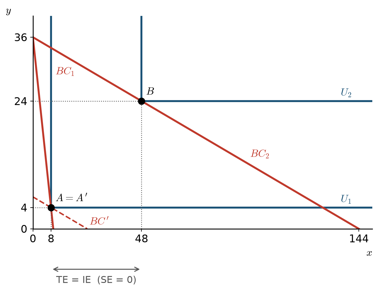
2.8 Substitution and income effects. Perfect complements: \(u = \min\left\{\tfrac13 x,\ \tfrac23 y\right\}\)
2.8.1 Initial bundle \(A\)
Evaluating the demand functions at \(p_x = 4\):
\[y_A = \frac{36}{2\cdot 4 + 1} = 4 \qquad\qquad x_A = \frac{2\cdot 36}{2\cdot 4 + 1} = 8\]
Initial utility:
\[U_1 = \min\left\{\tfrac13\cdot 8,\ \tfrac23\cdot 4\right\} = \tfrac83\]
2.8.2 Final bundle \(B\)
Evaluating the demand functions at \(p_x' = \tfrac14\):
\[y_B = \frac{36}{2\cdot \tfrac14 + 1} = 24 \qquad\qquad x_B = \frac{2\cdot 36}{2\cdot \tfrac14 + 1} = 48\]
2.8.3 Compensated bundle \(A'\)
Without wasting either good, with utility \(U_1 = \tfrac83\):
\[\tfrac13 x = \tfrac23 y = \tfrac83 \;\;\Longrightarrow\;\; x_{A'} = 8 \qquad y_{A'} = 4\]
Therefore:
\[A' = A\]
Income of \(BC'\):
\[\tfrac14\cdot 8 + 4 = 6\]
2.8.4 Substitution effect and income effect
\[SE = x_{A'} - x_A = 8 - 8 = 0\]
\[IE = x_B - x_{A'} = 48 - 8 = 40\]
\[TE = x_B - x_A = 48 - 8 = 40\]
2.8.5 Indifference curves and budget constraints