3 Step by Step: Short-Run and Long-Run Cost Functions
3.1 Setup
A firm produces \(q\) units of output using labor, \(L\), and capital, \(K\):
\[q = f(L, K)\]
The price of labor is \(w\) and the price of capital is \(r\):
\[w = 4 \qquad\qquad r = 1\]
The cost of producing with \((L, K)\) is:
\[TC = wL + rK\]
In the long run (\(lr\)) the firm chooses both \(L\) and \(K\). In the short run (\(sr\)) capital is fixed at \(\bar K\) and the firm chooses only \(L\):
\[\bar K = 8\]
Three technologies:
\[q = L^{1/3}K^{2/3} \qquad\quad q = \tfrac13 L + \tfrac23 K \qquad\quad q = \min\left\{\tfrac13 L,\ \tfrac23 K\right\}\]
3.2 Cobb-Douglas: \(q = L^{1/3}K^{2/3}\)
3.2.1 Short run: conditional labor demand
With \(\bar K = 8\):
\[\bar K^{2/3} = 8^{2/3} = 4\]
Substituting into the production function:
\[q = L^{1/3}\,\bar K^{2/3} = 4\,L^{1/3}\]
Solving for \(L\):
\[L^{1/3} = \frac{q}{4} \;\;\Longrightarrow\;\; L(q) = \frac{q^3}{64}\]
3.2.2 Short run: cost function
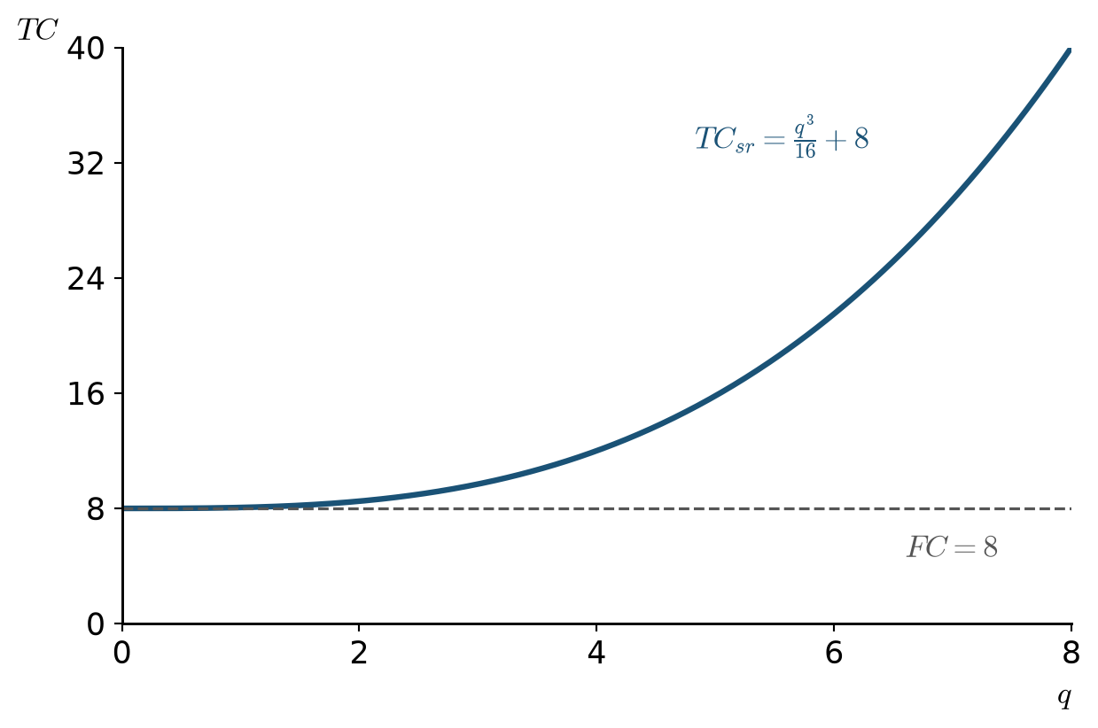
\[TC_{sr}(q) = w\,L(q) + r\,\bar K = 4\cdot\frac{q^3}{64} + 1\cdot 8\]
Simplifying:
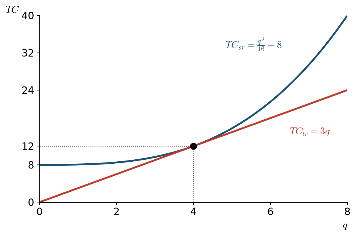
\[TC_{sr}(q) = \underbrace{\frac{q^3}{16}}_{VC}\; +\; \underbrace{8}_{FC}\]
3.2.3 Short run: marginal cost and average cost
Differentiating \(TC_{sr}\):
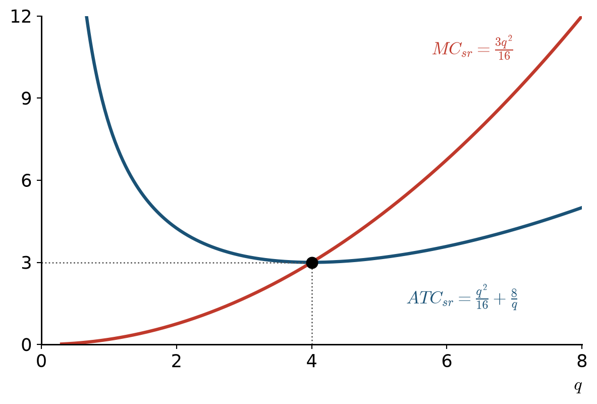
\[MC_{sr}(q) = \frac{dTC_{sr}}{dq} = \frac{3q^2}{16}\]
Dividing \(TC_{sr}\) by \(q\):
\[ATC_{sr}(q) = \frac{TC_{sr}}{q} = \frac{q^2}{16} + \frac{8}{q}\]
Minimum of \(ATC_{sr}\):
\[\frac{dATC_{sr}}{dq} = \frac{q}{8} - \frac{8}{q^2} = 0 \;\;\Longrightarrow\;\; q^3 = 64 \;\;\Longrightarrow\;\; q = 4\]
Evaluating at \(q = 4\):
\[ATC_{sr}(4) = 1 + 2 = 3 \qquad\qquad MC_{sr}(4) = \frac{3\cdot 16}{16} = 3\]
3.2.4 Long run: tangency condition
Marginal products:
\[MP_L = \tfrac13 L^{-2/3}K^{2/3} \qquad\qquad MP_K = \tfrac23 L^{1/3}K^{-1/3}\]
Dividing:
\[MRTS = \frac{MP_L}{MP_K} = \frac{K}{2L}\]
Setting it equal to \(w/r\):
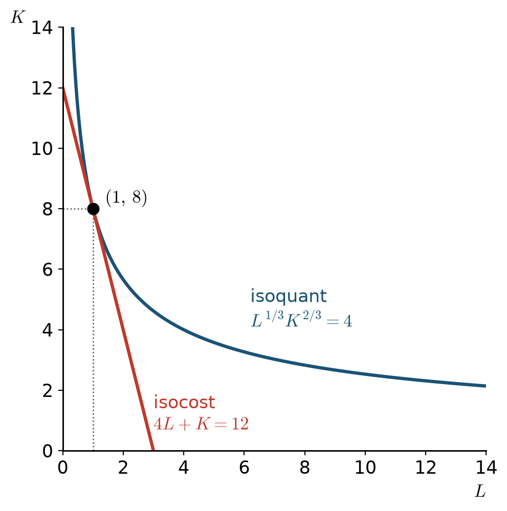
\[\frac{K}{2L} = \frac{4}{1} \;\;\Longrightarrow\;\; K = 8L\]
3.2.5 Long run: conditional factor demands
Substituting \(K = 8L\) into the production function:
\[q = L^{1/3}(8L)^{2/3} = 4L\]
Solving:
\[L(q) = \frac{q}{4} \qquad\qquad K(q) = 8\,L(q) = 2q\]
3.2.6 Long run: cost function
\[TC_{lr}(q) = w\,L(q) + r\,K(q) = 4\cdot\frac{q}{4} + 1\cdot 2q\]
Simplifying:
\[TC_{lr}(q) = 3q\]
Marginal cost and average cost:
\[MC_{lr}(q) = 3 \qquad\qquad ATC_{lr}(q) = 3\]
3.2.7 Isoquant and tangent isocost
For \(q = 4\):
\[L(4) = 1 \qquad K(4) = 8 \qquad TC_{lr}(4) = 12\]
3.2.8 Short-run and long-run cost functions
3.2.9 Returns to scale
\[f(tL,\,tK) = (tL)^{1/3}(tK)^{2/3} = t^{1/3+2/3}\,L^{1/3}K^{2/3}\]
Therefore:
\[f(tL,\,tK) = t\,f(L,K)\]
The technology exhibits constant returns to scale.
3.3 Perfect substitutes: \(q = \tfrac13 L + \tfrac23 K\)
3.3.1 Short run: conditional labor demand
With \(\bar K = 8\):
\[q = \tfrac13 L + \tfrac23 \bar K = \tfrac13 L + \tfrac{16}{3}\]
Solving for \(L\):
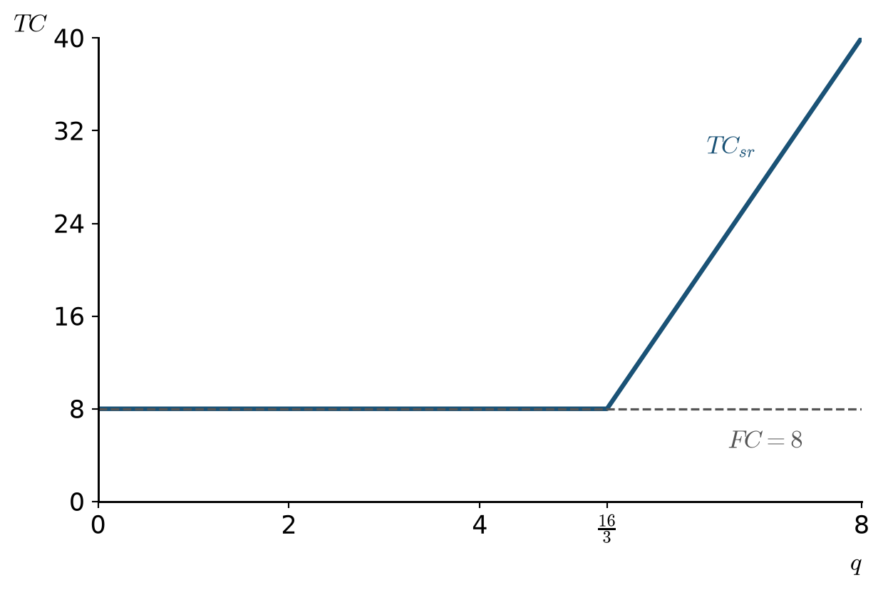
\[L(q) = \begin{cases} 0 & q \le \tfrac{16}{3} \\[4pt] 3q - 16 & q > \tfrac{16}{3} \end{cases}\]
3.3.2 Short run: cost function
\[TC_{sr}(q) = w\,L(q) + r\,\bar K = 4\,L(q) + 1\cdot 8\]
Substituting \(L(q)\):
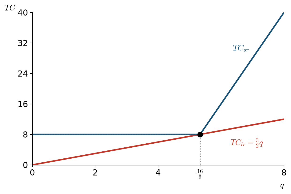
\[TC_{sr}(q) = \begin{cases} 8 & q \le \tfrac{16}{3} \\[4pt] 12q - 56 & q > \tfrac{16}{3} \end{cases}\]
3.3.3 Short run: marginal cost and average cost
Differentiating \(TC_{sr}\):
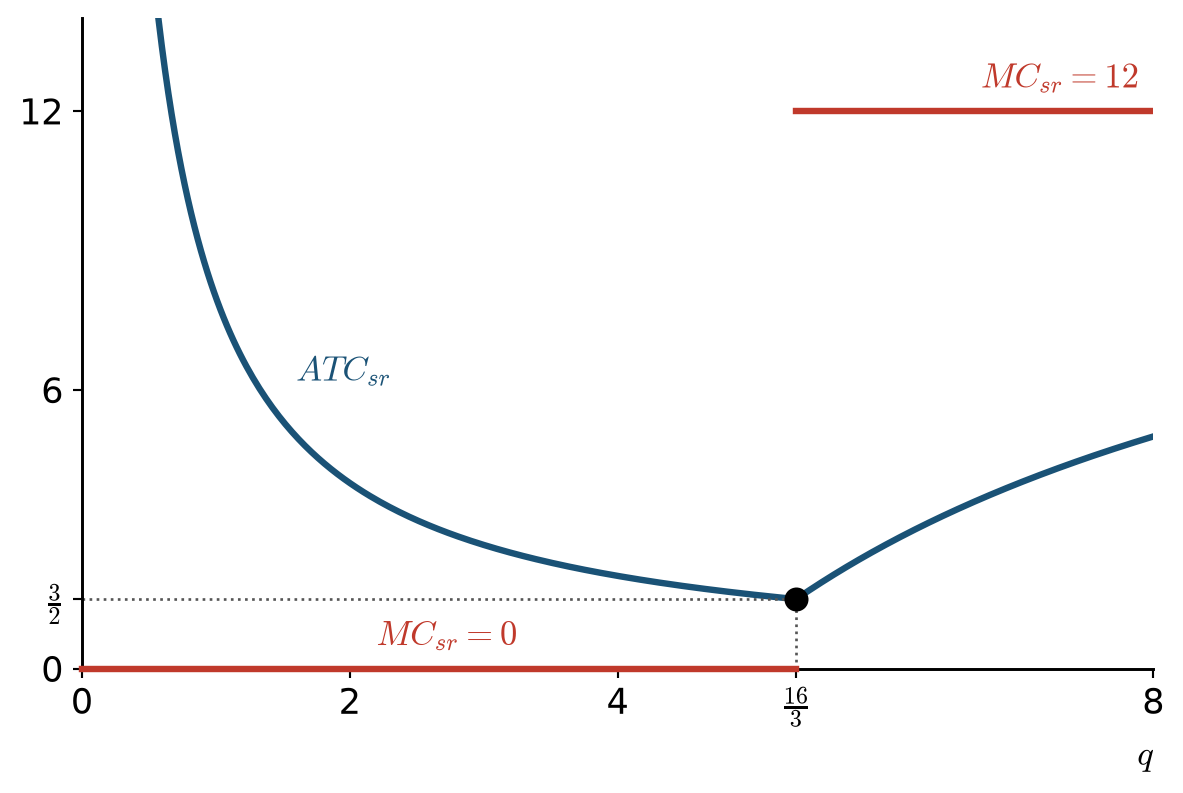
\[MC_{sr}(q) = \begin{cases} 0 & q < \tfrac{16}{3} \\[4pt] 12 & q > \tfrac{16}{3} \end{cases}\]
Dividing \(TC_{sr}\) by \(q\):
\[ATC_{sr}(q) = \begin{cases} \dfrac{8}{q} & q \le \tfrac{16}{3} \\[8pt] 12 - \dfrac{56}{q} & q > \tfrac{16}{3} \end{cases}\]
Minimum of \(ATC_{sr}\), at \(q = \tfrac{16}{3}\):
\[ATC_{sr}\left(\tfrac{16}{3}\right) = \frac{8}{16/3} = \frac32\]
3.3.4 Long run: comparing \(MRTS\) and \(w/r\)
Marginal products:
\[MP_L = \tfrac13 \qquad\qquad MP_K = \tfrac23\]
Dividing:
\[MRTS = \frac{1/3}{2/3} = \frac12 \qquad\qquad \frac{w}{r} = 4\]
Comparing:
\[MRTS < \frac{w}{r} \;\;\Longrightarrow\;\; L = 0\]
3.3.5 Long run: conditional factor demands
Substituting \(L = 0\) into the production function:
\[q = \tfrac23 K\]
Solving:
\[L(q) = 0 \qquad\qquad K(q) = \tfrac32 q\]
3.3.6 Long run: cost function
\[TC_{lr}(q) = w\,L(q) + r\,K(q) = 4\cdot 0 + 1\cdot\tfrac32 q\]
Simplifying:
\[TC_{lr}(q) = \tfrac32 q\]
Marginal cost and average cost:
\[MC_{lr}(q) = \tfrac32 \qquad\qquad ATC_{lr}(q) = \tfrac32\]
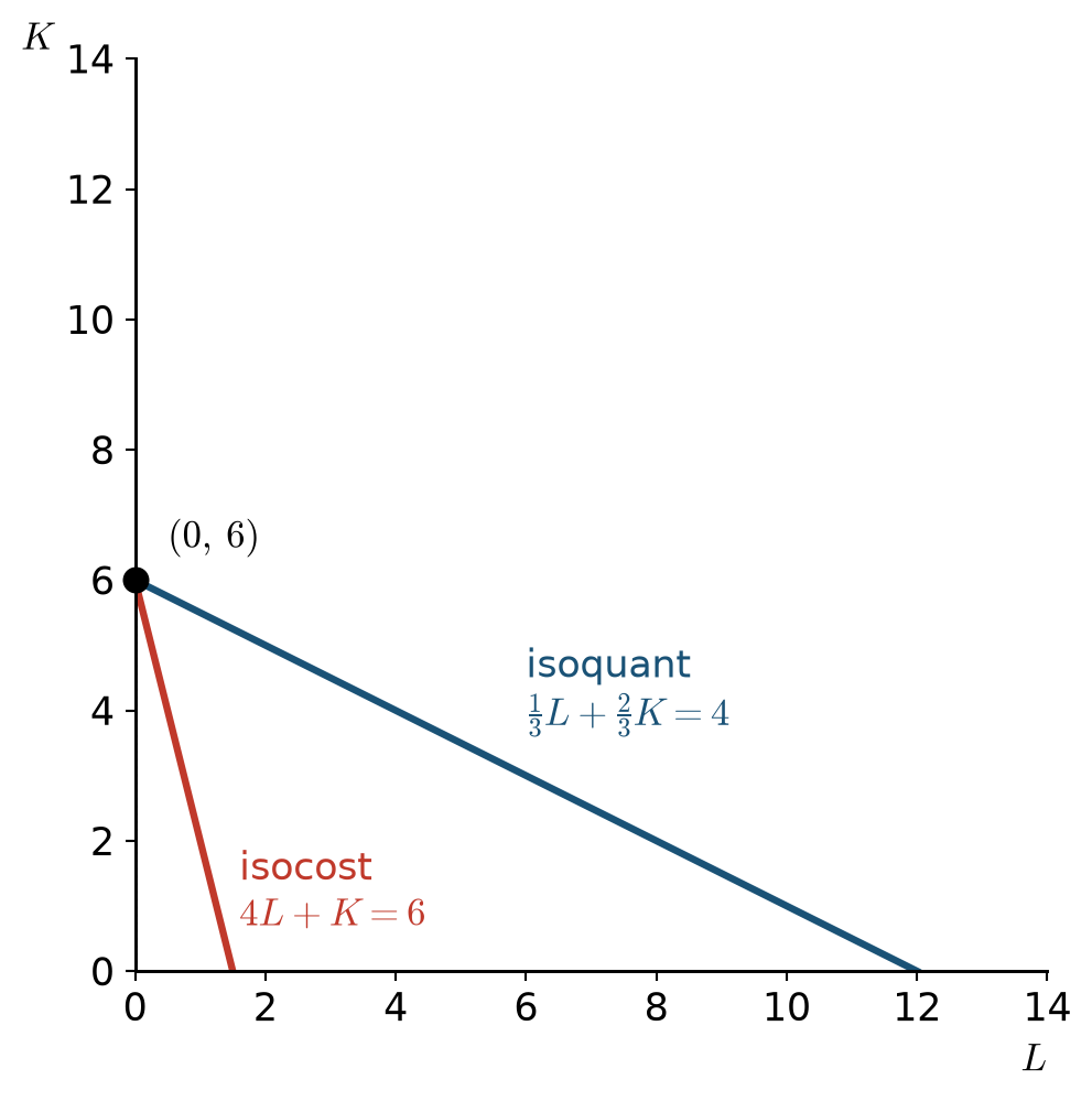
3.3.7 Isoquant and isocost
For \(q = 4\):
\[L(4) = 0 \qquad K(4) = 6 \qquad TC_{lr}(4) = 6\]
3.3.8 Short-run and long-run cost functions
3.3.9 Returns to scale
\[f(tL,\,tK) = \tfrac13 (tL) + \tfrac23 (tK) = t\left(\tfrac13 L + \tfrac23 K\right)\]
Therefore:
\[f(tL,\,tK) = t\,f(L,K)\]
The technology exhibits constant returns to scale.
3.4 Perfect complements: \(q = \min\left\{\tfrac13 L,\ \tfrac23 K\right\}\)
3.4.1 Short run: conditional labor demand
With \(\bar K = 8\):
\[q = \min\left\{\tfrac13 L,\ \tfrac23 \bar K\right\} = \min\left\{\tfrac13 L,\ \tfrac{16}{3}\right\} \;\;\Longrightarrow\;\; q \le \tfrac{16}{3}\]
Solving for \(L\):
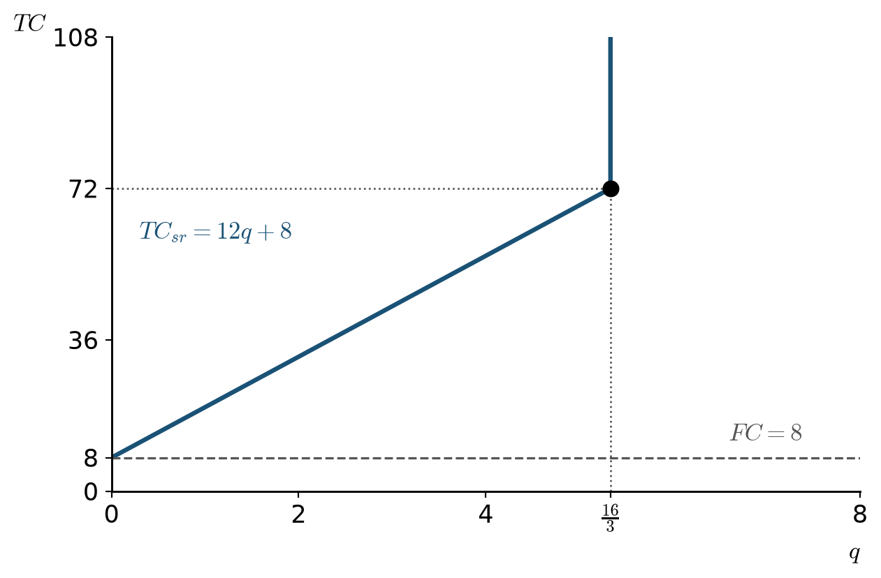
\[L(q) = 3q \qquad \left(q \le \tfrac{16}{3}\right)\]
3.4.2 Short run: cost function
\[TC_{sr}(q) = w\,L(q) + r\,\bar K = 4\cdot 3q + 1\cdot 8\]
Simplifying:
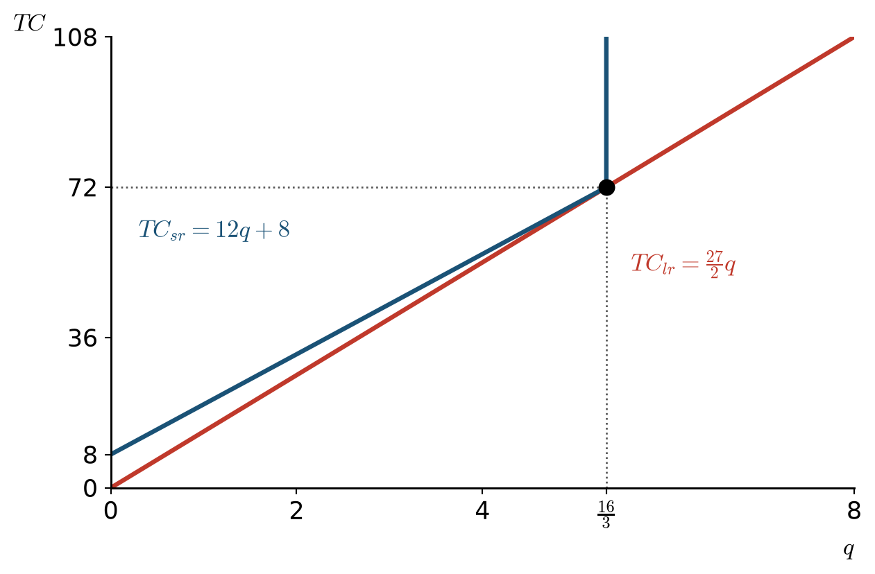
\[TC_{sr}(q) = \underbrace{12q}_{VC}\; +\; \underbrace{8}_{FC} \qquad \left(q \le \tfrac{16}{3}\right)\]
3.4.3 Short run: marginal cost and average cost
Differentiating \(TC_{sr}\):
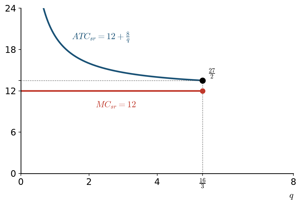
\[MC_{sr}(q) = 12 \qquad \left(q \le \tfrac{16}{3}\right)\]
Dividing \(TC_{sr}\) by \(q\):
\[ATC_{sr}(q) = 12 + \frac{8}{q} \qquad \left(q \le \tfrac{16}{3}\right)\]
Minimum of \(ATC_{sr}\), at \(q = \tfrac{16}{3}\):
\[ATC_{sr}\left(\tfrac{16}{3}\right) = 12 + \frac{8}{16/3} = \frac{27}{2}\]
3.4.4 Long run: conditional factor demands
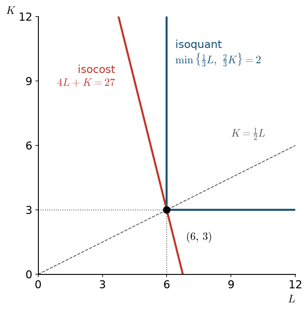
Wasting neither input:
\[\tfrac13 L = \tfrac23 K = q\]
Solving:
\[L(q) = 3q \qquad\qquad K(q) = \tfrac32 q\]
3.4.5 Long run: cost function
\[TC_{lr}(q) = w\,L(q) + r\,K(q) = 4\cdot 3q + 1\cdot \tfrac32 q\]
Simplifying:
\[TC_{lr}(q) = \tfrac{27}{2}\, q\]
Marginal cost and average cost:
\[MC_{lr}(q) = \tfrac{27}{2} \qquad\qquad ATC_{lr}(q) = \tfrac{27}{2}\]
3.4.6 Isoquant and isocost
For \(q = 2\):
\[L(2) = 6 \qquad K(2) = 3 \qquad TC_{lr}(2) = 27\]
3.4.7 Short-run and long-run cost functions
3.4.8 Returns to scale
\[f(tL,\,tK) = \min\left\{\tfrac13 tL,\ \tfrac23 tK\right\} = t\,\min\left\{\tfrac13 L,\ \tfrac23 K\right\}\]
Therefore:
\[f(tL,\,tK) = t\,f(L,K)\]
The technology exhibits constant returns to scale.